Peterson Barney Data

---

Reference

G. Peterson and H. Barney, "Control methods used in a study of vowels," Journal of the Acoustical Society of America, vol. 24, pp. 175-184, 1952 .

Purpose

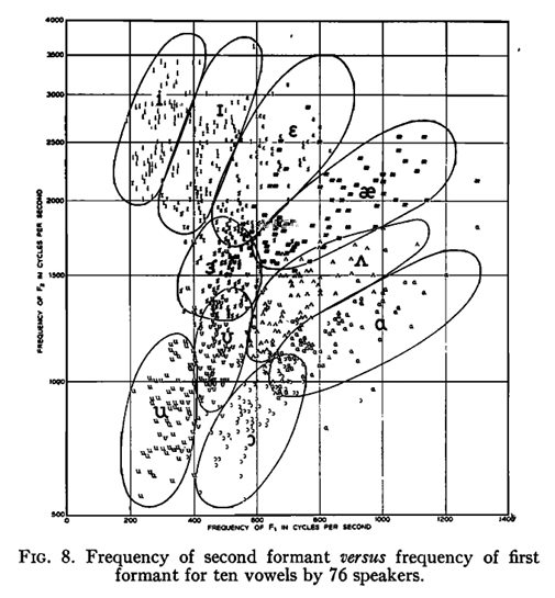
Especially Fig. 8 from this paper has become famous. In this notebook we try to recreate this plot, but also allow for slightly different implementation of statistics and visualization.

Disclaimers

• The original speech data was not preserved, but the formant measurements were. This data has been reused in a number of publications. I cannot guarantee that the dataset that I got is 100% correct as I don't remember exactly how I got them; I believe indirectly via Tony Robinson
• The average formant values obtained in this paper slightly deviate from the ones published in the 1952 paper, though the differences are barely significant. This is likely due to a slightly different frequency warping, numerical (rounding) errors, ...
• This data is much cleaner and more consistent than the data later collected by Hillenbrand (1995). So in a sense, this data looks too good to be true.

# uncomment the pip install command to install pyspch -- it is required!
#
#!pip install git+https://github.com/compi1234/pyspch.git
#
try:
    import pyspch
except ModuleNotFoundError:
    try:
        print(
        """
        To enable this notebook on platforms as Google Colab, 
        install the pyspch package and dependencies by running following code:

        !pip install git+https://github.com/compi1234/pyspch.git
        """
        )
    except ModuleNotFoundError:
        raise

# do all the imports and some generic settings
%matplotlib inline
import sys,os
import numpy as np
import matplotlib.pyplot as plt
import matplotlib as mpl
import pandas as pd
import seaborn as sns
import librosa
from copy import copy,deepcopy

import pyspch.core as Spch
import pyspch.display as Spd
#
np.set_printoptions(precision=2)
pd.options.display.float_format = '     {:.0f}  '.format
mpl.rcParams['figure.figsize'] = [8.,8.]
mpl.rcParams['font.size'] = 10
# get default color and marker orders for pyspch.display
markers = Spd.markers

Read the data

The full dataset contains 2 repetitions of each vowel by each speaker (33 men, 28 women and 15 children). You can select part of the data by setting the lists:

• gender: a list containing a selection of 'M','W','C'
• repetition: a list containing a selection of 1,2

Fig. 8 was constructed using genders=['M', 'W', 'C'] and repetition=[2]

Selecting all ADULT data is obtained by setting genders=['M', 'W'] and repetition=[1, 2]

file = 'https://homes.esat.kuleuven.be/~spchlab/data/PetersonBarney/peterson_barney_data.csv'    
genders = ['M','W','C']
repetition = [2]
vowels = ['IY','IH','EH','AE','AA','AO','UH','UW','AH','ER']
words = ["heed","hid","head","had","hod","hawed","hood","who'd","hud","heard"]
colors = ['blue', 'magenta', 'navy', 'cyan', 'green','limegreen','darkorange','red','brown', 'gold']
#
data_raw = pd.read_csv(file,sep=';')
data = data_raw.loc[:,["vowel","gender","F1","F2","F3"]]
data = data[data['gender'].isin(genders)]
data = data[(data.index%2+1).isin(repetition)]
# make sure that our categorical classes always appear in the same order for summarization/visualization
data['gender'] = pd.Categorical(data['gender'], categories = genders , ordered = True ) 
data['vowel'] = pd.Categorical(data['vowel'], categories = vowels, ordered = True) 
#
vowel2color = dict(zip(vowels,colors))
color2vowel = dict(zip(colors,vowels))
cmap = sns.color_palette(colors)
sns.set_palette(cmap)

Frequency Transformation to be applied to F2 and F3

In the Peterson Barney paper F1 is shown on a linear scale and F2 on a warped frequency scale. Details on the warping are not given in the paper. Most likely an early version of the 'mel-scale' was used. Here we use the mel scale as implemented in HTK which is a reasonable match. We apply the transformation both to F2 and F3 before computing averages or plotting. The axis labels is in Hz for easy interpretation. Below set SCALE to 'HTK' for this transformation; set it to 'LINEAR' for maintaining linear frequency. In summary we found that for these experiments the differences are quite limited.

SCALE = 'HTK'
def f2m(f):
    if SCALE == 'HTK':
        return(librosa.hz_to_mel(f,htk=True))
    else: 
        return(f)
def m2f(m):
    if SCALE == 'HTK':
        return(librosa.mel_to_hz(m,htk=True))
    else:
        return(m)

# set up default yticks for the F2 axis
yticks = np.array([750,1000,1500,2000,2500,3000,3500])
yticks_l= f2m(yticks)
ytick_labels = ["750","1000","1500","2000","2500","3000","3500"]
ylim = [500,3900]
xlim = [100,1500]

# add the transformed data as extra columns to the DataFrame
data['F2t']=f2m(data['F2'])
data['F3t']=f2m(data['F3'])

Compute average Formant Values

The computations are done gender independent and gender dependent The 'F2t' and 'F3t' values contain the averages computed in the transform domain. The 'F2' and 'F3' values are 'F2t' and 'F3t' reconverted to Hz

formants_gd = data.groupby(by=["vowel","gender"]).mean().unstack()
formants_all = data.groupby(by=["vowel"]).mean()
# add the example words to the table
formants_all.insert(0,"word",words)
formants_all.set_index(['word'],append=True,inplace=True)
formants_gd.insert(0,"word",words)
formants_gd.set_index(['word'],append=True,inplace=True)

# to view F2t reconverted to Hz
formants_all['F2'] = m2f(formants_all['F2t'])
formants_all['F3'] = m2f(formants_all['F3t'])
formants_gd['F2'] = m2f(formants_gd['F2t'])
formants_gd['F3'] = m2f(formants_gd['F3t'])

display(formants_all.loc[:,["F1","F2","F3"]].T)
display(formants_gd.loc[:,["F1","F2","F3"]].T)

vowel	IY	IH	EH	AE	AA	AO	UH	UW	AH	ER
word	heed	hid	head	had	hod	hawed	hood	who'd	hud	heard
F1	301	432	590	806	831	600	477	352	725	508
F2	2637	2292	2153	1947	1186	909	1143	943	1339	1537
F3	3220	2923	2857	2737	2704	2664	2591	2569	2687	1869

	vowel	IY	IH	EH	AE	AA	AO	UH	UW	AH	ER
	word	heed	hid	head	had	hod	hawed	hood	who'd	hud	heard
	gender
F1	M	265	385	526	665	719	575	439	303	636	489
	W	309	439	612	860	852	588	475	370	760	502
	C	368	524	689	1014	1035	677	563	424	854	563
F2	M	2295	1981	1837	1720	1085	842	1023	865	1189	1349
	W	2785	2472	2330	2046	1220	915	1156	937	1400	1632
	C	3203	2716	2602	2312	1358	1054	1410	1137	1584	1812
F3	M	2944	2548	2475	2396	2435	2402	2249	2232	2383	1689
	W	3304	3065	2993	2851	2811	2737	2675	2660	2772	1952
	C	3724	3588	3559	3370	3153	3161	3296	3245	3275	2142

marker_size = 20
PLT_TEXT = True
#
fig1,ax = plt.subplots(figsize=(7,7))
if PLT_TEXT: marker_size = 0
sns.scatterplot(ax=ax,x='F1',y='F2t',data=data,hue="vowel",marker='D',s=marker_size,hue_order=vowels)
if PLT_TEXT:
    for i,entry in data.iterrows():
        vow = entry['vowel']
        ax.text(entry['F1'],entry['F2t'],vow,ha='center',va='center',fontsize=5,color=vowel2color[vow] )
ax.set_yticks(yticks_l,ytick_labels)
ax.set_xlim(xlim)
ax.legend(loc='upper left', bbox_to_anchor=(0.82,1));
ax.set_xlabel('F1 (Hz)')
ax.set_ylabel('F2 (Hz)')
ax.set_title('Peterson Barney F1-F2 data');

Gaussian Modeling and Confidence Ellipses

Gaussian modeling is a standard and intuitive approach for scatter data as observed in the Peterson Barney data.
We show the data with a number of confidence ellipses; values selected are 1.0, 1.5 and 2.0. The Gaussian model may not be perfect, but it does a more than decent job. The 2*sigma contours are a sensible approximation of the region wherein Formants of a specific vowel are expected to appear.
Small variants are made of this plot: just the confidence ellipses, the mean values added to them and the mean values per gender added to the plots. The latter shows considerable variation between male and female values (due to vocal tract length differences) and it also draws our attention to the underlying bimodal distribution of the data.

# add confidence ellipses to previous plots
fig2 = deepcopy(fig1)
ax = fig2.get_axes()[0]
xfeat = 'F1'
yfeat = 'F2t'
sigmas = [1, 1.5, 2.0]
for vow in vowels:
    vowdata = data.loc[ data['vowel'].isin([vow]) ]  
    for sig in sigmas:
        Spch.plot_confidence_ellipse(vowdata[xfeat], vowdata[yfeat], ax, n_std=sig, edgecolor=vowel2color[vow] )
ax.set_title('F1-F2 data with Gaussian density estimates');
#
display(fig2)

# add average formant values to the plot
fig3 = deepcopy(fig2)
ax = fig3.get_axes()[0]
sns.scatterplot(data=formants_all,ax=ax,x='F1',y=formants_all['F2t'],
                hue='vowel',hue_order=vowels,s=100,legend=False)  
fig3

# add average formant values BY GENDER to the plot
fig3b = deepcopy(fig2)
ax = fig3b.get_axes()[0]
sns.scatterplot(data=formants_gd.stack(),ax=ax,x='F1',y='F2t', 
                hue='vowel',hue_order=vowels,style="gender",s=100,legend=False)  
ax.set_title('F1-F2 data with mean values per gender');
fig3b

Kernel Density Estimates

It is clear that our Gaussian Density estimates of the Formant distributions don't match well with the per formant 'regions' drawn in the paper We may assume that these were drawn by hand and inspired by a motivation to come up with maximally non overlapping F1-F2 regions Here we use Kernel Density plots that are more suitable to model data that is not Gaussian.
We played a bit with the control parameters and this is the best we could come up with. For some regions, like 'IY' and 'IH' the results are quite good. However the same parameters don't seem to work well for e.g. the 'AE' region . Also the overlap of the 'UW' vs 'UH' and 'AA' vs 'AO' is significantly larger than in the PB plots, which hints as a bias in the human interpretation of the results in the PB paper.

#
fig4 = deepcopy(fig1)
ax = fig4.axes[0]
sns.kdeplot(data, x="F1", y="F2t",hue="vowel", ax=ax, hue_order=vowels,levels=[ 0.35 ],bw_adjust=1.8,legend=None)
ax.set_title('Peterson Barney F1-F2 data with Kernel Density Estimates');
fig4

# convert the full notebook
! jupyter nbconvert PetersonBarney.ipynb --to html

[NbConvertApp] Converting notebook PetersonBarney.ipynb to html
[NbConvertApp] WARNING | Alternative text is missing on 5 image(s).
[NbConvertApp] Writing 1150873 bytes to PetersonBarney.html

# save selected figures
#fig1.savefig("../figures/pb_fig1.png")
#fig2.savefig("../figures/pb_fig2.png")
#fig3.savefig("../figures/pb_fig3.png")
#fig3b.savefig("../figures/pb_fig3b.png")
#fig4.savefig("../figures/pb_fig4.png")